
Radio Direction Finding
Britain’s secret eyes beyond its coasts that fed critical information to the Dowding System.
The Birth of RDF

Robert Watson-Watt
The entire air defense of Great Britain hinged on experimental technology called Radio Direction Finding (RDF). Today we know it as RADAR, its American name, but it was invented by the British, and without it the Dowding System would not have worked.
Radio Direction Finding works on the principal that if metal objects reflect radio waves. The RAF began investigating this concept in the 1930’s in hopes of building an EMF “death ray” to destroy incoming bombers. In January 1935, the head of the National Physical Laboratory’s Radio Department, R.A. Watson Watt was consulted about using electromagnetic radiation to damage aircraft or kill the crew. The RAF was asking for a “death ray” straight out of science fiction. After preliminary calculations, he realized that the power requirements were too high to make a practical weapon. But he, like many scientists around the world, realized that he could use EMF radiation to detect incoming aircraft.
In February of 1935, Dowding funded an experiment by Watson Watt to test this concept. Although the experiment design was crude, and used existing BBC radio signals rather than transmitting their own , the results were promising. Sensing the potential, Dowding petitioned the Air Ministry to fund development. Although there is a common belief that the Air Ministry was unenthusiastic and agreed to developing Dowding’s RDF if the towers would not interfere with grouse hunting, the truth is that the Daventry experiment led to a massive program to build a network of RDF stations around England’s southeastern coast. The program enjoyed widespread support within the Air Ministry and access to generous funding.(1) The RAF worked with contractors to build a network of stations covering the Thames estuary, which became the nucleus of the larger Chain Home (CH) defense system that would grow to over 50 stations before the end of the war. The early stations were the AMES-1 stations, whose technical specifications and operation is described below.

RDF Transmitters (left) and Receiving Antennae (right) at Poling. © IWM CH 15173
How RDF Worked
Although the British were the first to deploy an operational radar network, their technical solution was based on an approach that would become a technical dead end. Unlike modern radar systems, early RDF systems did not transmit a targeted, rotating beam. Instead, RDF stations transmitted a pulsed radio wave from fixed vertical towers that “painted” an area roughly 100 degrees in front of the tower. These radio waves bounced off incoming aircraft and the reflected EMF energy was detected by a series of receiving antennas located several hundred yards from the transmitters. These radio transmissions traveled in a wide “spotlight” beam pattern because, unlike modern radar, these stations would not rotate. Because they could only “sense” in one direction, Dowding placed his stations on the coast, pointed out to sea.
Inside an operator’s hut, an RDF Operator watched the signal trace, a green horizontal line on a Cathode Ray Tube (CRT). When the RDF station receivers detected a reflection from an aircraft, a pattern appeared in the trace, called an “echo.”
Technical specs
Although there were many configurations deployed during the war, the typical AMES-1 RDF station had the following characteristics:
Frequency: 20-30 MHz
Peak Power: 350 kW
Height: Transmitters - 360 ft, Receivers - 240 ft
Pulse Repetition Frequency (p.r.f): 25 and 12 p.p.s.
Determining Location
A plastic scale attached to the CRT marked the distance away from the station in miles. Where the echo occurred on the trace indicated the range of the incoming aircraft. Range measurements were typically accurate, but because RDF transmitted a floodlight beam, bearing readings were not precise. To determine the echo’s bearing the RDF Operator used a goniometer, which was mechanically connected to the dipoles on the receiver antennae. By turning the goniometer dial back and forth, the RDF Operator determined the echo’s bearing from the station. The Operator would swing the goniometer and note when the trace reached its “minimum,” which indicated the bearing to the incoming aircraft. Operators used the minimum because it gave a sharper indication than other methods. When the incoming signal was weak, Operators instead used the “maximum” and corrected the indicated bearing by 90 degrees.(2)

RDF Operator looking at the CRT. Note the goniometer to her left. © IWM CH 15332
Determining Number of Aircraft
RDF stations were also capable of providing rudimentary information about the number of aircraft they were detecting. The shape of and number of peaks in the trace provided a rough picture of the number and formation of aircraft. If planes were more than 1.5 miles apart, they’d appear as separate peaks.(3) If the formations were tighter, the peaks would merge, making identification more difficult. To assist with counting, the Operator was able to shorten the transmitted pulse from 20 to 6 microseconds, which improved range detection 3:1.(4) Converting the trace into a reliable picture of raid strength was called, “counting the beats.” This practice was highly subjective and required experience.
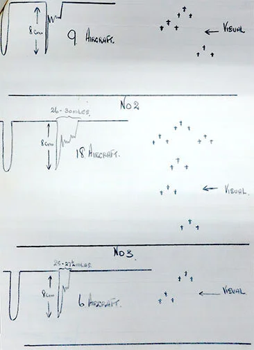
Sketches showing how different formations and numbers appear on the CRT echo trace (AVIA 7 212).
Accurate counting was an ongoing problem throughout the battle. Underestimations were common with inexperienced RDF Operators. These mistakes led Controllers to scramble insufficient numbers of fighters for larger raids. During the war, the RAF never solved the problems associated with counting.

July 24th memo from Keith Park documenting problems with counting aircraft (AVIA 7 212)
Determining Altitude
The RDF Operators also tried to determine the altitude of incoming aircraft. This was critical, because in a dogfight altitude is advantage. But because RDF was rudimentary technology, accurately gauging height was difficult. The design of the RDF transmitters used a series of dipoles at different heights. Height finding used the goniometer to compare the signal received between the 215’ dipole and the 95’ dipole. The Operator would swing the goniometer using the same technique as determining bearing. Early in the war, the Operators would take readings and use a calibrated table to convert the number to altitude. This method was superseded by the “Fruit Machine,” a complex analog calculator built by Siemens, which converted input from the goniometer into a map grid reference and altitude reading respectively.(5)
Even with the best performance by the Operator, RDF height measuring had several technical limitations. The primary consideration was the elevation angle between the station and the aircraft, which constrained the accuracy of altitude measurements. The early CH stations were only capable of reliable reporting height between 1.5 and 6 degrees. If the elevation angle was less than 1.5 degrees, the Operator would indicate the altitude as if it was at 1.5 degrees, regardless of the actual angle. In practice, this meant that altitude was over-reported at long distances. The converse of this situation was the greater danger. As the angle increased above 6 degrees, the Operator would sense the height as if it was 4 degrees. This “turning over” of the height curve meant that the altitude would be under-reported. And because the elevation angle would increase as an aircraft approached the station, this became a grave situation.(6) Unfortunately, this was not a problem that could be solved through experience or training. This was a technical limitation of the system. Although inaccurate, CH stations were reporting the best information physically possible. This limitation was fixed during later CH deployments, when additional aerials increased the upper limit angle of elevation to 15 degrees. This did not make the height reading more accurate, but greatly reduced the range where “turning over” was a problem.
To make matters even worse, the AMES-1 stations were not just inaccurate in height reporting. Height reading experiments also uncovered a fundamental weakness with early stations: they had sensing blind spots for low flying aircraft and could not detect aircraft below 5,000 ft.
Test Your Air Defense Skills
Operate a Chain Home Radar Station
This simulation recreates the experience of using an AMES-1 Chain Home station, Britain's early warning radar system during the Battle of Britain. Between one and five German aircraft are approaching England's coast, and it's your job to locate them.
How to Use the Radar
Watch the CRT screen for aircraft echoes, which appear as peaks in the horizontal line
Use the Goniometer Angle slider to sweep back and forth until you find these echoes
Sweep back and forth and watch the echo shape. When an echo reaches its maximum height, note the goniometer angle - this gives you the bearing
Record the range by reading the horizontal scale across the top of the CRT
Reporting to the Dowding System
By determining both bearing and range, you're providing crucial information that the entire air defense network needs to coordinate fighters and antiaircraft defenses.
Realistic Limitations
This simulation includes authentic limitations of wartime radar:
Aircraft may initially be invisible due to range or altitude constraints
Raiders will gradually appear on the trace as they approach your station
Some aircraft may remain undetected if flying too low
Click "See what the RDF is seeing" to view a table and map of the incoming raids and compare with your findings.
Chain Home
Dowding recognized that because RDF was experimental, it had considerable weaknesses. So he deployed the stations in a network. The concept was that by using readings from multiple stations, the inaccuracies in their readings would be cancelled. Multiple wrongs making a right.
He organized the stations in a chain, placing each station 20 km apart. Any one station’s beams overlapped with its neighbors, so several RDF stations would detect the same incoming planes. This network, named Chain Home, became the backbone of Britain’s early warning system. By the outbreak of war there were 18 Chain Home stations, but the network eventually expanded to include 50 stations. Like almost any feature of the Dowding System, the Chain Home network was not homogeneous. As experiments led to development, later stations had different technical specifications and configurations, For example, the stations on the western approaches were different than the eastern approaches, some stations had “all-round-looking” transmitters, and some were buried emergency backup transmitters.(7)
Chain Home Low
To address the weaknesses detecting aircraft flying lower than 5,000 feet, the RAF deployed a second type of RDF network: Chain Home Low. When activated in 1940, the Chain Home Low network addressed the vulnerabilities with Chain Home. RAF scientists based its design on Naval gun-laying radar. These units used a revolving, narrow beam, like modern radar. This characteristic made Chain Home Low more accurate at determining bearing, but its effective range was shorter, making it inadequate to replace Chain Home. Because its design did not use multiple stationary dipoles, Chain Home Low stations were not capable of estimating altitude.
The RAF experimented with how to process information from both station types. Ultimately they decided that Chain Home Low information would pass through a neighboring Chain Home station. This became a logistical challenge for both the RDF Operators and the Filter Room personnel.
(1) Neale, B.T. “CH - The First Operational Radar." The GEC Journal of Research. Vol 3. No. 2. 1985.
(2) Ibid.
(3) AVIA 7 212: Counting of Aircraft
(4) Neale, B.T. “CH - The First Operational Radar." The GEC Journal of Research. Vol 3. No. 2. 1985.
(5) Ibid.
(6) AVIA 7 183: Programme of Research Work - General Operations Rooms - RDF Filter Room
(7) Neale, B.T. “CH - The First Operational Radar." The GEC Journal of Research. Vol 3. No. 2. 1985.